Engineering formulas

cadagent.formulas holds the closed-form equations that 3D-printed mechanisms keep needing: beams and snap arms, torsion bars, springs, screws, four-bar linkages, wall conduction and fan operating points. Agents call it from Python instead of re-deriving the equations. The website's demonstrations call a browser port of the same functions, and the two are tested against one set of golden vectors, so a demo never shows a number an agent would not get. Every function states its SI units and its validity limits, and cites its source by author, title, edition and section.

Try it: the snap-arm explorer

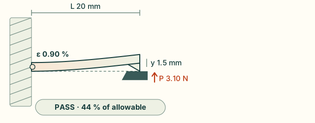
The explorer (<cad-cantilever>, also on Snap fits) runs the browser port of snap_arm. Sliders set the length, root thickness, width and deflection, and you pick the material and print direction. The beam bends along its computed curve, coloured by strain, with the root strain, force and pass or fail against the filament's allowable strain.

Snap-arm explorer, before its controls load: a CoPA arm 20 mm long, 1.6 mm thick at the root and 6 mm wide, bent 1.5 mm at the hook along its computed curve; root strain 0.90 %, 44 % of the 2.02 % allowed along the layers, a pass; force 3.10 N

Limits

A closed form is not proof of fit or strength. Each result holds only inside the limits it states. A printed part is weaker across its layers than any isotropic formula assumes, and creeps under a held load. Print the part and measure it.
Small deflection and linear elasticity. These hold for every beam, torsion and spring formula here. For large deflections, contact or plastic strain, use FEA (cadagent.simulation.fea) and a test.
Screws. Torque gives preload to about ±25 % even with a known nut factor; in plastic the factor is unknown until measured. Thread stripping assumes even load sharing, which real threads do not have.

Why it is built, not adopted

We looked before writing anything. Each closed form here is a few lines long. The browser has to compute exactly what the Python does, and a Python dependency cannot be mirrored in a web page. CI's core job installs only PyYAML and NumPy. So the equations are written out here and tested against their sources. Beyond them, use fluids and ht for duct losses and convection, pint for unit-checked quantities, SymPy to derive new closed forms, and pylinkage for linkage synthesis.

The projects we surveyed, and what is reused from this repo

fluids and ht by Caleb Bell (MIT): pipe and duct losses, fittings, and hundreds of convection correlations. When a design needs a Nusselt number or a duct loss coefficient, use them. ht.conduction.k_to_R is the same plane-wall resistance as wall_resistance here. Our composite wall with surface films follows the same series-resistance layout as ht's cylindrical version.
pint (BSD-3) for callers who want unit-checked quantities. These functions take plain SI floats, so the browser port can match them.
SymPy (BSD-3) for deriving new closed forms. The tapered-arm integrals here were done by hand and checked numerically in the tests.
pylinkage (MIT) for linkage synthesis and optimisation; here only position analysis.
me-toolbox (MIT, by Omri Stein) for Shigley-style springs, fasteners and fatigue. It was read for scope. Its author describes it as a personal tool, and it pulls in SymPy.
Reused from this repo, never forked:
- The snap-arm functions call cadagent.mechanical.compliant.snapfit, so they match cad-agent snapfit exactly.
- The demo's materials come from cadagent.mechanical.compliant.allowables.
- The straight-line fan curve is the same model as cadagent.thermal.heatsink.FanCurve. A test checks that the two solvers find the same operating point.

How the sources, the Python, the golden vectors and the browser port connect:

flowchart TD
    S["Books, guides, standards<br/>Roark · Shigley · Covestro · Norton<br/>Incropera · White · ISO 68-1, 898-1"] --> P["cadagent.formulas<br/>(Python, SI, cited)"]
    C["cadagent.mechanical.compliant<br/>snapfit · allowables"] --> P
    P --> A["agents<br/>catalogue() · snap_arm() …"]
    P --> V["tools/formula_vectors.py<br/>golden vectors · demo materials"]
    V --> J["kit/formulas.js<br/>(browser port)"]
    J --> D["&lt;cad-cantilever&gt;<br/>on Snap fits"]
    classDef here fill:#fffdf5,stroke:#173d3c,color:#173d3c
    classDef near fill:#eef1e4,stroke:#6f8a80,color:#173d3c
    classDef out fill:#ffe1cc,stroke:#bd3a12,color:#173d3c
    class P,V,J here
    class S,C near
    class A,D out

What it computes

SI units throughout: metres, newtons, pascals, kelvin, watts, radians, m³/s. A strain is a fraction (0.02 = 2 %).

All 36 functions in catalogue(): what each computes, its source and where it is valid

Function	What	Source	Valid within
`rect_second_moment`	I = b h³ / 12	Roark 8th ed., Table A.1	solid rectangle
`cantilever_tip_deflection`	y = F L³ / 3 E I	Roark 8th ed., Table 8.1, case 1a	Euler–Bernoulli, small deflection
`beam_stiffness`	3, 12, 48, 192 E I / L³ (cantilever, guided, simply supported, fixed–fixed)	Roark 8th ed., Table 8.1	point load; slender beam
`cantilever_shape`	the deflected curve, constant or tapered arm	Roark 8th ed., Section 8.1, integrated exactly	end load
`cantilever_strain_profile`	surface strain along the arm over the root's	Roark 8th ed., Section 8.1 (σ = M c / I)	end load
`cantilever_thickness_profile`	thickness along the arm (design 2 tapers to h/2)	Covestro guide, Table 1	linear taper
`cantilever_taper_factor`	exact k in y = k ε L² / h: 2/3, 1.0904, 0.8552	Roark, integrated; Covestro Table 1 prints 0.67, 1.09, 0.86	rectangle
`snap_root_strain`	ε = y h / (k L²), the guide's factors	Covestro guide, Table 1 (via `snapfit`)	small deflection, one part rigid
`snap_deflection_force`	P = (b h² / 6) Es ε / L	Covestro guide, Table 1 (via `snapfit`)	secant modulus at that strain
`snap_arm`	strain, force, stiffness, pass/fail, permissible deflection	Covestro guide, Table 1 (via `snapfit`)	a pass has no extra margin
`shear_modulus`	G = E / 2(1 + ν)	Roark 8th ed., Section 2.2	isotropic only
`torsion_constant_round`, `torsion_constant_rect`	K for solid, hollow and rectangular bars	Roark 8th ed., Table 10.1 (solid and hollow concentric circular, solid rectangular sections)	Saint-Venant torsion; the rectangle within 0.5 %
`torsion_shear_stress_round`, `torsion_shear_stress_rect`	peak shear stress	Roark 8th ed., Table 10.1	away from ends and steps
`torsion_bar_twist`, `torsion_bar_stiffness`	θ = T L / K G, T / θ = K G / L	Roark 8th ed., Section 10.1	constant section
`spring_index`, `spring_rate`	C = D / d, k = G d⁴ / 8 D³ Na	Shigley 10th ed., Sections 10-1, 10-3, Eqs. (10-1), (10-9)	4 ≤ C ≤ 12; 15–85 % of travel
`bergstrasser_factor`, `spring_shear_stress`	K_B = (4C + 2)/(4C − 3), τ = K_B 8 F D / π d³	Shigley 10th ed., Sections 10-1, 10-2, Eqs. (10-5), (10-7)	static, round wire
`preload_from_torque`, `torque_for_preload`	F = T / K d, with `NUT_FACTORS`	Shigley 10th ed., Section 8-8, Eq. (8-27), Table 8-15	±25 % at best
`nut_factor`	K from thread and collar friction	Shigley 10th ed., Section 8-8, Eq. (8-26)	60° thread
`tensile_stress_area`	As = π/4 (d − 0.9382 p)²	ISO 898-1:2013; Shigley Table 8-1	ISO metric
`thread_shear_areas`, `thread_strip_force`	0.75 π D1 Le (screw), 0.875 π d Le (hole)	ISO 68-1:1998 basic profile	even load sharing, no tolerances
`grashof`	Grashof class, whether the input crank turns fully	Norton 5th ed., Chapter 2	rigid links
`fourbar_angles`	coupler and output angles, open or crossed	Freudenstein (1955); Norton 5th ed., Chapter 4	position only; a gap under 1e-12 of the longest link counts as closed
`transmission_angle`	angle between coupler and rocker	Norton 5th ed., Chapter 4	position only; the same closing test
`wall_resistance`, `film_resistance`	R = L / k A, R = 1 / h A	Incropera 7th ed., Section 3.1.2, Eqs. (3.6), (3.9)	steady, 1-D
`wall_heat_flow`	layers and films in series: heat flow and every face temperature	Incropera 7th ed., Section 3.1.3	no contact resistance
`fan_curve_line`, `system_coefficient`	the datasheet fan line; k in Δp = k Q²	White 7th ed., Section 11.5	same air density
`fan_operating_point`	fan curve against Δp = r Q + k Q², solved exactly per segment; flags a stall dip	White 7th ed., Section 11.5	steady flow

fx.catalogue() returns the same list as data, with each function's units, limits and full citation, so an agent can find the formula it needs without reading the source.

from cadagent import formulas as fx
arm = fx.snap_arm(length=0.020, thickness=0.0016, width=0.006, deflection=0.0015,
                  modulus=2.703e9, allowable_strain=0.020)       # CoPA, along the layers
arm["strain"], arm["force"], arm["passes"]                        # 0.0090, 3.1 N, True
fx.preload_from_torque(torque=0.5, diameter=0.003)                # 833 N with K = 0.2
fx.fan_operating_point(fx.fan_curve_line(15.2, 0.0108), k=2e6)   # flow, pressure, stability

In the browser, kit/formulas.js exports the functions the demos use (snapArm, cantileverShape, cantileverStrainProfile and the others in the golden vectors) in the same SI units.

Tests that keep it honest

tests/test_formulas.py checks each function against a published value or an independent derivation written out in the test.

What each family is tested against: beams, torsion, springs, screws, linkages, heat and air

Beams.
- Beam stiffness by the direct stiffness method.
- The tapered-arm curves by numerical integration, and the Covestro Table 1 factors as the exact integrals rounded.
- Example I of the guide in SI units, and agreement with cad-agent snapfit to 1e-12.
Torsion.
- Rectangular sections against the Saint-Venant series (within 0.5 %, the worst at aspect 1.145), and against the tabulated coefficients in Shigley, Section 3-12.
- The guide's torsion snap as the same mechanics.
Springs.
- The rate derived from the wire as a torsion bar.
- Bergsträsser against Wahl.
Screws.
- The ISO stress areas against their tabulated values.
- K ≈ 0.2 from Eq. (8-26) at a friction of 0.15.
- The 0.75 and 0.875 shear-area factors derived from the ISO 68-1 profile.
Linkages.
- Loop closure, and an independent circle-intersection construction, at every input angle.
- Kites (a = b, c = d) and near-kites, every 0.1 degree, where the textbook root divides 0 by 0.
- Parallelograms and other change-point linkages, every 0.1 degree and every 1e-9 rad near 0 and 180 degrees, where the two branches meet and round-off can push the discriminant below 0. Each branch must be the one asked for.
- The input's limit angles on linkages whose crank cannot turn fully, where the linkage closes in one position.
- Norton's Example 4-1.
Heat and air.
- The composite wall face by face.
- The fan point against the quadratic root and against cadagent.thermal.heatsink.operating_point.
- A stall dip flagged unstable.

tools/formula_vectors.py --check fails when the committed golden vectors or the demo's material table no longer match the Python. tests/webkit-formulas.test.mjs runs the browser port on those vectors to 1e-12.